The “AVAIL” Availability Calculator will help help you to analyse the availability performance of networks
made up of components with occasional random failures followed by restorations with random durations.
Within that sort of environment, would you believe that the following situations are all possible, even if unusual:
Two different systems that have the same numerical value of Avaliability may have such radically different properties
that some customers would reject the first and accept the second, whilst other customers would reject the second and insist on the first.
Normally a backup link improves the availability and reliability performance of telecommunications system. But starting with a single telecommunications cable,
and then adding a second physically diverse backup link in parallel, the failure rate may get WORSE rather than better.
Usually we would expect that adding an unreliable system in series makes overal performance worse,
but it is possible that a system which currently fails to meet customer requirements can be “IMPROVED” by adding an unreliable component in series,
to the extent that it meets all customer requirements.
The longer we live, the older we get (of course), meaning that the more lifteime we accumulate behind us the less our expected remaining lifetime becomes.
But it is possible that the longer a fault has been resisting attempts to fix it, the “younger” it gets,
in the sense that its expected remaining time-to-repair increases.
By mastering a few simple equations – in fact by using a spreadsheet to perform the calculations for you – you will be able to explain those paradoxes, and calculate the availability of compound
(but not too complicated) systems from the properties of their individual components.
Security is hard – really hard. SHA256 is generally taken to be very secure, however
checking SHA sums relies on the assumption that a miscreant has not hacked my web site,
replaced the zip file with a zipped spreadsheet containing malware, and re-computed both hashes,
then edited this page to show the new hashes.
To the best of my knowledge that is no more likely to have happened to this web site than to many others you probably trust.
In any case, you also need to trust that I have not included malware in the spreadsheet myself – maliciously or inadvertently.
I assure you I have not done so maliciously, and I am confident I have not done so inadvertently because
my students at the University of Melbourne have used it for many years with no complaints.
If you have any remaining doubts, check my Linkedin page.
I look really honest. Even without a neck-tie.
And many people, including many students, have joined my network.
Download then uncompress the Zip file, then open the Excel Workbook. You will see the dialog box:
The Availability Calculator relies on Excel Macros, so click on “Enable Macros", since I am now a fully trusted source.
The workbook opens on the first sheet “Availability and Reliability", which is considered “Home". Altogether there are 16 sheets:
Availability and Reliability (Home)
Availability
Failures
Restoration
Availability Units
Failures Units
Restoration Units
Components
Series
Series Graph
Parallel
Parallel Graph
Calculator
Networks
Problems
The Next Challenge
From the Home sheet you can progress through most of the workbook by using the buttons labelled with “ > ”, “Previous”, “Next”, and “Home”, or specific links like “Go to Calculator”.
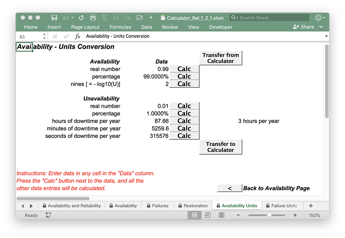
The “Units” sheets for Availability, Failures, and Restorations allow conversions between different ways of expressing those quantities.
For example, a motor car may be unavailable for an average of six hours per year; a bus service may have three “nines” availability – which has the better availability?
Of course this calculation is trivial, but having a servant to perform the arithmetic will be useful for more complicated problems. To answer this particular question, click your way to “Availability Units” (or just select the tab of that sheet at the bottom of the workbook). You will see this screen:
Following the instructions in red, enter the value 6 in the Data column next to the label “hours of downtime per year”
(the cell presently contains the value 87.66).
Press Enter, then click on the Calc button right next to the value you just entered.
All the other entries will be updated. The car has availability, as a real number, of 0.999315537
(don't worry that the precision is a bit excessive!).
The Unavailability (defined as 1-Availability) is a bit less than 0.001 or 10^-3.
Hence the number of “Nines” (defined as -log(Unavailability)) is a bit greater than 3,
so the car beats the bus, in this example.
Both of the other “Units” sheets work in much the same way.
Tehcnically speaking the terms “year,” “month,” “week,” “day,” “hour,” and “minute” are not Scientific units of time.
The Scientific time unit is the second, the definition of which you may read about in Wikipedia.
Those other units, which we use every day, are defined legally rather than scientifically.
Every now and again, standards authorities around the world agree to add a leap-second into our lives,
making the minute, hour, and so on vary by plus one second.
From time to time some administrations add or subtract an hour so we can enjoy the sunshine better.
Hence “one day” may be 23, 24, or 25 hours.
Of course the number of days per month is not constant, and even the number of days in a year varies.
For engineering purposes, when I refer to one minute, I mean 60 seconds, not 60 or 61.
One hour is 60 minutes and a day is 24 hours. Now comes the tricky bit.
What is a month? Well I just shut my eyes and call it 30.5 days on average.
For one year, I use 8766 hours which is 365.25 days.
You may consider this a bit sloppy, especially if you are a Mathematician or Scientist,
in which case I invite you to consider the best achievable accuracy of measurement of
an Average Time to do Anything in Particular (see A Note About Accuracy).
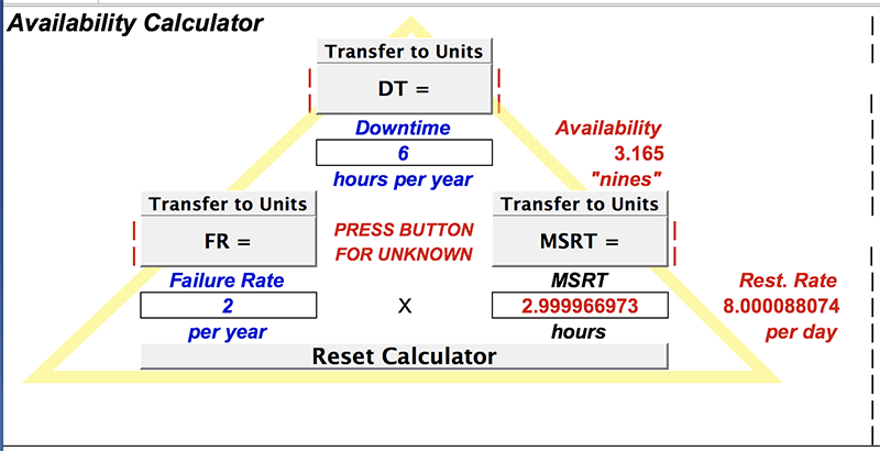
The main sheet in the workbook is the Calculator, so before leaving the Availabiity Units sheet,
press on the button labelled “Transfer to Calculator". You should see this:
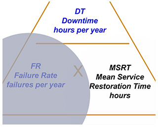
The Calculator is triangular in shape, based on a simple mnemonic. The three quantities, Average Downtime per year, or DT;
Failure Rate in failures per year, or FR; and Mean Service Restoration Time (MSRT), in hours, are related by the simple equation:
DT = FR × MSRT
If you are given any two quantities, the third is easily calculated.
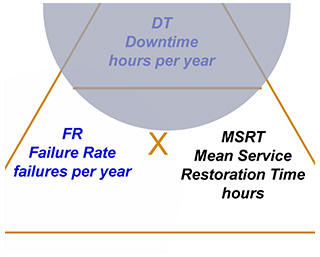
For example, if you cover the top of the triange you will see the equation for DT as a function of the other two, like this:
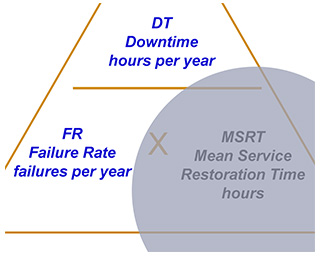
But what if it is MSRT that we consider to be “unknown”?
Just cover the unknown and you will be reminded of the right equation. In this case
MSRT = DT / FR
Which can be seen here:
Likewise, covering the “FR” corner of the triangle, we see the pattern:
FR = DT / MSRT
From the Availability Units page we transferred in the value of DT as 6 hours per year. However, the three values are out of kilter.
To fix that, we need to press the button corresponding to the “unknown quantity”.
Let's say it is MSRT that is unknown, so click on the button “MSRT =”.
You should be expecting the value 3 hours to appear – hopefully it does.
Now the three quantities are “in kilter,” and the red warning has disappeared.
What if we have two similar motor cars in parallel – many households have two or more cars.
Of course, in the case of scheduled maintenance we could make sure one car was always available.
However, that is not the situation analysed here.
It is essential to note that we assume all failures are random, and all restoration times are random also.
In fact we assume that both are (Negative) Exponential Random Variables with some known Mean Value.
Furthermore we will assume that all components are statistically independent.
If the first car is down that tells us nothing about the other car – it may be up or down at random,
just as it is when the first car is up instead of down.
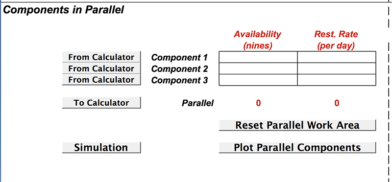
To estimate how two cars would work for us, on the Calculator sheet, move down to the Parallel Work Area. It looks like this:
To load it up with two copies of our car, click on “From Calculator” next to “Component 1”, then again,
click on “From Calculator” next to “Component 2”.
Don't go crazy and click again or you could have three cars in the Parallel work area – leave Component 3 blank.
Now click on “To Calculator" to return the two-car-combination as a single component in the Calculator.
We can see the MSRT is now 1.5 hours – a nice convenient figure – but why is it precisely half the value for a single car?
Also, it turns out the Failure Rate is now 0.002737851 (again – don't worry about the excessive precision),
but is that good or bad. Clearly it is an improvement, but by how much?
Click on “Transfer to Units” above the Failure Rate to convert into more meaningful units.
The answer appears in multiple different units now – the one I can relate to is a mean time to failure of 365.25 years.
So with two random, independent, and identical cars we have a situation of no car available for an average of
one and a half hours every 365 years or so, on average.
Of course, cars don't last 365 years, but if there were 365 identical instances of the same situation,
we would expect about one outage per year across all 365 instances.
But what if you need to drive to the bus-stop and then catch a bus (with three nines availability, and assume two hours MSRT).
You have two cars to choose from, but now the bus service is in series with the two-car-combo.
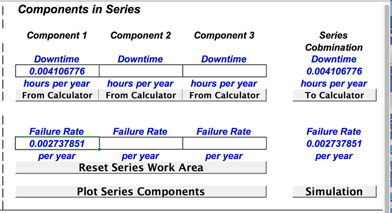
Go back to the calculator, and transfer the two-car-combo into the Series Work Area to the right of the Calculator (on the same sheet).
Click on the first “From Calculator” button. It should look like this – showing the numbers that refer to the two-car-combo:
Now return to the main part of the Calculator and enter the parameters of the bus service: 3 nines unavailability
(I recommend using the Availability Units Sheet to convert 3 nines to average Downtime per year of 8.766 hours),
and 2 hours MSRT (assumption).
Press on the button to calculate the unknown Failure Rate. I get 4.383 failures per year
(one every eighty three and a third days, on average – pretty awful).
Transfer the answer into the Series Work Area as the second component, then transfer the result back to
the main part of the Calculator by pressing “To Calculator”
(the process analogous to the one for the Parallel Work Area).
The final result is that by using the two-car-combo to get to the bus stop, then relying on the bus to get the rest of the way,
the failure rate is one failure per 83.28 days, and the MSRT is 119.98 minutes or one hour fifty-nine minutes and
fifty-nine seconds approximately – just about exactly the same as the bus service on its own!
You experience almost exactly the same availability service as someone living right at the bus stop – why is it so?
Of course the calculations performed are quite simple – you can do them by hand if you prefer,
but I find the spreadsheet quicker than manuual calculation after a little practice.
The formulas used depend on the assumptions of:
All times are Negative Exponential
All random variables are independent
In the event of multiple failures, there is no resource constraint – teams always work concurrently at full strength
The model applies only for “small" values of Unavailability.
For example, if two elements both have Unavailability greater than about 10%,
we cannot use the formulas in the Calculator for series networks.
These are assumptions of convenience, meaning that the results should be taken as somewhere between indicative and authoritative,
depending on circumstances. The Calculator is a tool, not a master.
Understanding those limitations, following are the formulas used for series and parallel combinations.
If two components are in series, then an outage of either one implies an outage of the network. We assume that:
The total number of failures per period of time is the sum of the two individual numbers of failures.
This ignores the possibility that one component may fail while the other is already down.
Hence it relies on the assumption of “small” Unavailability
The total amount of downtime in any time period is the sum of the individual downtimes.
Again, this relies on the assumption of “small” downtime.
So for series combinations, we assume we can add the individual FR values, and add the individual DT values.
This is how the Series work area of the Calculator works.
This also allows us to plot the results graphically.
On a chart of FR versus DT, each component is represented by a point.
Joining the point to the origin gives us a vector.
The series combination of a number of components is represented by the vector sum of the components,
on the chart of FR versus DT (See the Series Graph Sheet).
Quick Quiz to see if you have mastered the concept: If you start with a single component,
with known FR, DT, and MSRT, and then add another component in series,
two of the three parameters must get worse, but
the third one may get better, or worse, or stay the same.
Which parameters are the ones that must get worse?
If two components are in parallel, then an outage of the network occurs only when both components are down concurrently.
We assume that:
The state of each component is independent of the state of any other component.
Therefore the Unavailability of the combination of two components is the product of the individual Unavailabilities.
When both components are down, two maintenance teams work to restore service on each component.
The first team to finish effectively restores service to the whole network.
Hence we need to analyse a “race” between two Negative Exponential Variables.
Ideally we would like to find parameters that are additive. Luckily there is one parameter in common use that fits the requirement.
If we have an Availability of, for instance, 0.999, that is often described as “Three Nines Availability”.
Mathematically, the value of “Nines” can be computed from
Nines = – log(Unavailability)
Well multiplying Unavailabilities is equivalent to adding Nines. For example, if we have two components wih
Availabilities of 0.99 and 0.999 then the Unavailabilities are 10-2 and 10-3, corresponding to 2 Nines and 3 Nines.
Multiplying the Unavailabilities gives us 10-(3+2) = 10-5 or 5 Nines Availability.
As to the race between two Negative Exponential Random Variables, we need the formula for the probability of
a restoration requiring time t or more. That will be of the form:
P{T>t} = e - r t
where r is termed the “rate” of the random variable. We will refer to it as the Mean Service Restoration Rate, or MSRR
The higher the value of MSRR the quicker the restoration, on average.
Please take it from me that the Mean Servce Restoration Time is inversely proportional to MSRR:
MSRT = 1/MSRR
You can verify this fact about Negative Exponentials in Wikipedia.
When we have a race bwteen two Negative Exponentials, the restoration time will be greater than t if and only if
BOTH Random Variables are greater than t. Relying on independence, we can calculate:
P{T>t} = e - r t e - s t
= e - (r+s) t
Examining ths equation, it is the same form as the equation for a single Exponential Random Variable.
Hence the winner of the race to restore service (whichever team it may be) has an Exponential distribution
with mean rate equal to the sum of the two individual mean rates.
Indeed this principle can be continued to three, four, or any number of teams all working in parallel
and all racing to restore service – the first one finished, out of however many are racing,
restores the service.
Hence Mean Service Restoration RATES are additive. It makes sense.
If two teams are both working at their normal rate concurrently,
the total rate of work is equal to the sum of the two rates.
So for parallel combinations, we assume we can add the individual Mean Service Restoration Rates, and add the individual Nines.
This is how the Parallel work area of the Calculator works.
This also allows us to plot the results graphically.
On a chart of MSRR versus Nines, each component is represented by a point.
Joining the point to the origin gives us a vector.
The parallel combination of a number of components is represented by the vector sum of the components,
on the chart of MSRR versus Nines (See the Parallel Graph Sheet).
Quick Quiz to see if you have mastered the concept: If you start with a single component,
with known FR, DT, and MSRT, and then add another component in parallel,
two of the three parameters must get better, but
the third one may get better, or worse, or stay the same.
Which parameters are the ones that must get better?
“Precision” refers to the number of decimal digits in our answers. “Accuracy” refers to how far
the answers lie from the truth.
Of course, showing a precision of six or seven significant figures in the answers is not meant as a
claim of that degree of accuracy.
The precision is used to allow follow-on calculations, such as subtracting two quantities that are very close.
So just how accurate are the numbers.
We can form a view on that by considering how much effort it would take to measure some of the variables.
All processes that require averaging across samples are subject to statistical variation.
For example, consider the measurement of a Mean Time to Restore Service.
Using Wikipedia again,
you will see that the variance of a Negative Exponential Variable is the square of its mean.
From your Statistics textbook you will know that if we average, for instance, one hundred
measurements of restoration times, which all have a true mean value of M,
the variance of the sample mean is
V = M2 / 100
The 95% Confidence Interval is calculated from the square root of the variance, and is approximately
M ±1.95 M / 10
So we can rely on the answer to within about plus or minus 20% – not particularly impressive accuracy.
Suppose we decide we want ± 1% accuracy – equal to one twentieth of the error range we get with a hundred samples.
To achieve that we need not twenty times but four hundred (twenty squared) times the number of measurements,
or 40,000 individual restorations.
If the restorations are expected to take about 3 hours,
we will need one repairperson for 120,000 working hours (equivalent to 62.5 years – well nigh impossible for one person)
or sixty two and a half staff for 1 year each, or some other combination.
Setting aside the expense, there is another problem:
we need to ensure that all of our sixty-two-and-a-half staff have identical skill levels,
and that none of our staff improve (or degrade) their skill level during the experiment.
They should all perform all restorations at the same skill level throughout the experiment, otherwise
we have one or multiple moving targets.
I would suggest that, except in exceptional circumstances, 1% accuracy is not attainable for any measured mean durations
for people to do something (including Mean Time to Restore and Mean Time to Fail).
In practice I think we would be lucky to get plus or minus 10%.
Considering that random tallys, such as the number of failures per period of time, are also subject to Statistical variation,
I would need convincing that we can know the availability of a real-world system to within better than 10% to 20% margin of error.
Of course we may still need better precision than that, especially if we are comparing two systems
on the basis of “everything else being equal”. Then we will want to know the hypothetical performance of each alternative
based on having precisely the same parameters (except for the parts that we choose to vary from one alternative to the other).
What is a component. Furthermore, what does it mean to consider series or parallel combinations of components.
It is a mistake to limit our thinking to one component corresponding to one physical entity in a network.
Rather, one component represents one failure mode of our system.
To illustrate the point, consider the example of a radio tower on a remote mountaintop.
Let's assume we have arranged for a commercial power supply, which is not perfectly reliable.
We may choose to have battery backup power.
Then we may consider all the equipment as “electronics”.
Finally, let's agree that the radio tower is at risk due to natural disturbances.
For the sake of illustration we will say that it may fail due to “lightning”.
To develop a model of our radio tower as a whole, we look at each possible failure mode.
The commercial power may fail, or the battery may fail. Only if both are down concurrently does our
radio tower lose power. Therefore we model those two failure modes as components in parallel.
Even with power available, the electronics may fail. Therefore we put the electronics component
in series with the parallel combination of battery and commercial power.
If our radio tower takes a direct lightning strike then all the other components are of no use.
Therefore we put a component called “lightning” in series with the rest.
It is obvious that our model is a logical model of the relationships between the parts.
Nothing – neither energy, nor matter, nor information – is expected to flow through our model network from one end to the other.
The model simply represents how the whole system may be either up or down depending on
the state of the components we chose to include in the model.
The component we labelled “lightning” should rather be called “freedom from outage due to lightning”.
We know (or guess, or assume) the mean time that our radio tower can enjoy such freedom.
We also know (or guess, or assume) how long it will take, on average, to restore service
after an event that deprives our radio tower of that particular freedom.
Sometimes we refer to the average time before a failure (or other event) as a “lifetime”.
It is a mistake to interpret this as the time taken for a component to get old and “die”.
Rather the “lifetime” is simply the inverse of the “rate” of dying.
Indeed, we assume all components we use are in their prime.
If they show signs of getting old, in the sense that they have a much greater risk of failure
in any given month, they are probably worth replacing with nice, young components,
hence disappearing from our model, and our consideration.
To illustrate this point about “lifetimes” consider the example of an adult human
selected at random from a population.
We may know from actuarial tables that such a person has the following death-rates per year
(these particular numbers are just made up for this illustration):
Accident
0.0010 per year
Cancer
0.0020 per year
Heart Disease
0.0025 per year
Other Diseases
0.0040 per year
All Other Causes
0.0100 per year
All these components should really be labelled “Fredom From ...”. For instance: “Freedom From Heart Disease”. “Freedom from Accident” has a Mean Failure Rate of 0.0010 failures per year.
This suggests an average of one millennium of life, free from accidents, lies ahead for our subject – but a thousand years of life for one individual is quite unrealistic.
In fact all these processes are engaged in a “race”.
Since they are in series, the first to fail brings down the whole system.
Just as in the case of parallel restorations, we can add the failure rates of series components
to find the equivalent rate for the winner, whichever process that may be.
In our example, the sum of all the rates is equal to 0.0195 per year.
The inverse of that rate is 51.3 years, approximately.
The correct conclusion is that our model human can expect, on average, a remaining lifetime
of about 51.3 years.
In summary, “lifetime” does not refer to ageing (such as the crumbling of optical fibre,
plastic becoming brittle and snapping, or people growing decrepit) – it is the inverse of the total rate of random failures that may occur whilst “in one's prime”.
If you work through the problems you will find the answers to two of the paradoxes above.
Normally, a backup link improves a telecommunications system, but starting with a single telecommunications cable,
and then adding a second physically diverse backup link in parallel, the failure rate may get WORSE rather than better.
Work through Problem 3 to see an example of this.
3. You are operating an international telecommunications service.
You use an undersea cable that fails once every three years and takes
three weeks to repair, on average.
Immediately it fails, you reserve capacity on a satellite, but it takes 2 hours, on average,
before you may
use your allocated capacity.
The satellite service fails once every 10 days and takes one hour to be restored.
Create a series/parallel network
to represent your service and hence calculate the overall performance.
Are outages purely random?
How would you manage communications
with your customers?
Let's ignore the part about “it takes 2 hours” before you can use the allocated capacity. We will come back to that part later.
I trust it is obvious that we have an undersea cable in parallel with a satellite service.
Entering the data into the Calculator (with the help of the Units Sheets), you should agree that the undersea cable
gives availability of about 1.72 Nines, and the Satellite about 2.38 Nines.
Adding the backup satellite to the undersea cable improves the Availability up to about 4.10 Nines.
Also the MSRT comes down from three weeks to about one hour. Both improvements are very significant.
But the Failure rate has gone UP from one per 3 years to one per 1.43 years – more than twice as bad as
the undersea cable on its own. Why is it so?
Hint: consider the performance of the satellite during the 21 days while the undersea cable is being restored.
Returning the the part about the 2-hour delay, I would add another component in series to the parallel combination,
with a failure rate of one per 3 years and a MSRT of 2 hours.
Although this would not give a faithful representation of the full system, it should give
numerical results that are “good enough”. Of course the failure rate will be even worse than before.
Also we can expect the MSRT to increase – but by how much?
Usually we would expect that adding an unreliable system in series makes overall performance worse,
but it is possible that a system that does not meet customer requirements can be “IMPROVED”
to the extent that it meets all customer requirements by adding an unreliable component in series.
Problem 5 gives an example where this seemingly crazy result is true, in theory.
It can cost approximately zero to add an unreliable series component to any system that is dependent on
electric power supplied through a plug and socket.
Simply set up two random processes that give alarms at random times.
You could set one to go off on average every year – when that alarm goes off pull out the power plug,
and start the second random alarm clock.
That alarm could be set to go off in one hour, on average.
When the latter alarm goes off put the power plug back in.
There you have it: a component that costs almost nothing, and generates failures at a rate of one per year,
with a MSRT of one hour.
Of course that is madness. Why would any engineer deliberately sabotage their own system at random like that.
IN THEORY, it can improve performance, only in a strictly theoretical sense. Problem 5 gives an illustration.
5. A customer specifies a service with maximum unavailability of 0.1 hours per year and a maximum MSRT of 3 hours.
Individual components have a failure rate of 8 per year and a MSRT of 12 hours.
You may build a network using components in parallel to deliver the required performance.
How many components in parallel are needed to meet the Unavailability target?
Does this meet the target for MSRT?
In an effort to meet the target values specified by the customer,
you add a component in series which has a MTBF of 33 years and a MSRT of 150 minutes.
Are all targets met now? Has the addition of this component really improved performance?
For the sake of discussion, assume each individual component costs a million dollars.
So the decision to use one more component requires consideration.
However, the “component in series which has a MTBF of 33 years and a MSRT of 150 minutes”
is the seemingly crazy process of two random alarm clocks and someone who is willing to pull the plug on the whole network – near enough to zero additional cost.
If you use the Calculator as I did, you will conclude that a network of three components in parallel meets
some of the requirements, but not all.
If you add another million-dollar component in parallel, all requirements will be met.
ALTERNATIVELY, you could add one of those “free components” in series.
Amazingly, with just three one-million-dollar components plus one free component,
ALL customer requirements are met,
as you will be able to verify using the Calculator. A saving of one million dollars!
Of course an Engineer would never use that as a solution – what would be a better way to proceed?
Hint: think about how a system with three components in parallel fails. First one component fails.
No need to panic – we still have two in parallel.
But then a second component fails while the first is still being restored.
Now we have two components down, and the service is dependent on just one component to keep going.
If the third component fails we will be plunged into emergency mode.
Service Restoration will become urgent!
Can you think of anything you could do to prepare for that emergency?
There is no single correct answer – it depends on the physical nature of the components.
The lesson here is that Engineers must treat their tools as servants, not masters.
Two different systems with the same numerical value of Avaliability may have such radically different properties that some customers would reject the first and accept the second,
whilst other customers would reject the second and insist on the first.
Of course the explanation lies in the fact that the two systems have different Failure Rate and Mean Time to Restore Service.
For example, assume System 1 has a Failure Rate of one per year and a MSRT of 30 seconds.
System 2 has a failure rate of one every 2,880 years and a MSRT of 24 hours.
Use the Calculator to check their Availabilities (should be equal). So, which system is better? Of course, it depends.
Suppose you are operating a commercial airline and all of your planes behave like System 1. Once per year every plane fails in mid air for 30 seconds.
The passengers experience a full half minute of virtual weightlessness. If you have a few hundred planes in your fleet, you can expect several such incidents per week.
Wouldn't you prefer a plane that lasts 2,880 years, on average?
On the other hand, suppose your company operates 2,880 elevators nationwide.
Suppose that once per year each elevator experiences a software glitch, and stays locked in place for 30 seconds – irritating, indeed.
Compare that with a set of elevators similar to System 2. About once per year one of your 2,880 elevators remains locked in place for 24 hours.
Your passengers in the elevator have to spend a full day in a prison of your making. TV cameras and news reporters arrive at the scene to record the drama.
A hole has to be made to pass in food and water. You are famous, but not in a good way.
Surely the frequent irritation of 30 second outages would be better?
The longer we live, the older we get (of course), meaning that our expected remaining time-to-live reduces.
But it is possible that the longer a fault has been resisting attempts to fix it,
the “younger” it gets, in the sense that its expected remaining time-to-repair increases.
The Negative Exponential random variable has the very special property that its mean time to persist is constant –
it is the only distribution with such a property. In fact, no matter how long it has been going,
it still has the exact same distribution of remaining time to go as it had when it commenced at time zero.
Think of a single radioactive atom with a half-life of one day.
It has probability one half of decaying spontaneously within one day.
But if it happens to be a “lucky” atom which survives one day,
then it has a probability of one half of decaying during the following day. And so it goes on.
No matter how long it survives, it has the same probabiility one half of decaying in the following day,
and hence the same mean-time-remaining-to-live that it started with.
It has no memory – it does not age –
it is neither “lucky” nor “unlucky” –
suddenly and unpredicatbly it simply passes to another state.
That is the way with Negative Exponential Random Variables.
I wouldn't like to have a Negative Exponential lifetime, even though it means never ageing.
A simple example where a random variable has increasing time to live would be a “Mixture Distribution”.
For example, suppose you are in charge of a communication link between Earth and Mars.
Let's assume all faults have Negative Exponential lifetimes, but there are two types of fault:
software faults with a one-hour MSRT, and hardware faults with a one-day MSRT – both random with Negative Exponential Distributions. Suddenly the channel goes silent.
Everything is good to go here on Earth, so the fault must be on Mars.
But what sort is it.
Of course, the channel you operate is the only channel between the two planets (let's assume),
so there seems to be no way of knowing.
Let's assume the different types of fault are equally likely,
so the time to restore service has an overall average of 0.5 times one hour plus 0.5 times one day,
or 12.5 hours, without knowing which type it is.
However, we do get some information as time goes by.
After three hours, it is more likely that the fault is hardware rather than software.
Only a very small fraction of software faults persist longer than three hours
(even taking into account the propagation time).
But the majority of hardware faults last longer than three hours.
If it is still not fixed after 24 hours we can just about rule out software problems.
Hence after 24 hours we are almost certain of a hardware fault, so the expected remaining time to restore service is 24 hours.
Whether we get to 36, or 48, or 72 hours without any success,
the expected remaining time to restore service is still 24 hours in every case!
In fact, the expected remaining time to restore service transitions smoothly from about 12.5 hours initially
up to a limit of 24 hours, the longer the fault persists.
If our lifetimes worked in similar fashion we might say: “the more we age, the younger we get”,
in the sense that the more years we have behind us, the more we can expect in front of us.
Here is a final puzzle for you. Suppose you have not merely two cars, but three cars.
If you go back to the Calculator and add a third car in parallel with the other two you should find a failure rate of one outage, with an average duration of one hour,
once every 3,118,535,181 years, approximately.
But do you really expect your three cars to last three billion years? Scientists assure us that within that time the Earth's magnetic field will surely fail
(slight exaggeration for emphasis). Surely you don't believe your three cars will outlast the Earth's magnetic field? Even if your cars are still functioning,
will there still be a bus service to convey you to your office?
It makes barely more sense to talk about 3.1 billion identical instances of three-car-combos.
Yes, if the cars can survive one year, then we have the equivalent of 9.3 billion “car-years” in just twelve months.
Surely the majority of the cars (and the Earth's magnetic field) can be relied on for that relatively trivial time.
Yes, in theory, if 3.1 billion families all were faced with the same situation we would expect, in theory, about one outage per year.
In reality, and I think this is the clue to the answer, other factors would arise and swamp
the purely random failures we have assumed in our lovely mathematical model.
In the case of a single instance of a three-car-combo considered over 3 billion years, the failure rate of the components will
change with time – presumably increasing asymptotically to 1 as the centuries go by.
Even without considering the aging of components,
riots, political upheavals, earthquakes, extreme weather events, and many other factors could come into play.
By analysing our three-car-combo in isolation we have tacitly assumed that “nothing else can go wrong”.
In general, Mother Nature (or is it “Ms Nature”) rarely has the grace to follow any of my models – no matter how elegant they are.
So what is a reasonable interpretation of your extreme numerical result? I invite you to ponder that, as I will.
A related question: is the improvement due to the third car sufficient to justify, economically,
the cost of ownership of another car (for three billion years)?
For that matter, was the upgrade from a one-car family to a two-car family worth it in terms of improved car availability.
Of course, availability is not the main reason why a family would invest in a second car.
But what if you are operating a satellite sevice.
Is the second hundred-million-dollar satellite good value for money as a backup for the first? This thought leads on to the topic of "Avail-o-nomics".
I hope you enjoy exploring the Availability Calculator, now that you know how to use it.
Having mastered the basic calculations of Availability and Reliability, the time has come to consider whether it is all worth it.
Click on the link below to proceed to the Avail-o-nomics section of the ARC web site.